Correlation and Regression Analysis in Excel with Examples

What is Correlation and Regression?

• Correlation: Measures the strength and direction of the relationship between two variables. Values range from -1 (perfect negative) to +1 (perfect positive).
• Regression: Helps predict the value of a dependent variable (Y) based on an independent variable (X). It gives a mathematical equation for the relationship.

---

Example Dataset

Year	Ad Budget ($)	Revenue ($)
2020	5000	100000
2021	7000	120000
2022	8000	140000
2023	9000	160000
2024	10000	180000

---

Step 1: Calculate Correlation in Excel

1. Use the CORREL Function:
   • Formula: =CORREL(B2:B6, C2:C6)
   • B2:B6: Ad Budget range.
   • C2:C6: Revenue range.
2. Result:
   • Correlation Coefficient: 1.0
   • Interpretation: A perfect positive correlation (ad budget and revenue move together).

---

Step 2: Perform Regression Analysis in Excel

Steps to Run Regression:

1. Enable the Analysis ToolPak:
   • Go to File > Options > Add-ins.
   • Select Analysis ToolPak and enable it.
2. Open Regression Tool:
   • Go to Data > Data Analysis > Select Regression.
3. Input Ranges:
   • Input Y Range: C2:C6 (Revenue).
   • Input X Range: B2:B6 (Ad Budget).
4. Check Options:
   • Check “Labels” if you included headers.
   • Select the output range or a new worksheet.
5. Click OK to generate the regression output.

---

Interpreting Regression Output:

1. Key Values:
   • Intercept: 80000
   • Slope: 10
   • Regression Equation: Revenue = 80000 + 10 * Ad Budget
2. Use the Equation:
   • Predict revenue for an ad budget of $11,000: Revenue = 80000 + 10 * 11000 = 190000

---

Visualization:

• Create a Scatter Plot with Trendline:
  1. Highlight the dataset.
  2. Go to Insert > Scatter Chart.
  3. Add a Trendline:
     • Right-click a data point, select Add Trendline.
     • Check “Display Equation on Chart” to see the regression line equation.

---

Insights from the Example:

1. Correlation: Strong positive relationship between ad budget and revenue.
2. Regression: Provides a predictive model for revenue based on ad budget.
3. Visualization: A scatter plot with a trendline makes it easier to understand the relationship.

Sample Output

SUMMARY OUTPUT

Regression Statistics
Multiple R 0.986393924
R Square 0.972972973
Adjusted R Square 0.963963964
Standard Error 6003.002252
Observations 5

This is the output of a Linear Regression Analysis performed in Excel, likely using the “Data Analysis Toolpak.” It includes several key components that summarize the regression model, its significance, and the relationship between the independent variable (X Variable 1) and the dependent variable.

Key Sections Explained:

1. Regression Statistics:
   • Multiple R: Measures the correlation between the observed and predicted values. Here, it’s 0.9864, indicating a very strong positive correlation.
   • R Square: Indicates how much of the variation in the dependent variable is explained by the independent variable(s). Here, it’s 0.973 (or 97.3%), meaning most of the variance is explained.
   • Adjusted R Square: Adjusts R Square for the number of predictors. It accounts for potential overfitting in multiple regression.
   • Standard Error: Measures the accuracy of the predictions. A lower value indicates better fit.
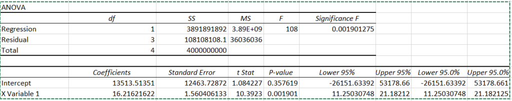
2. ANOVA (Analysis of Variance):
   • df (Degrees of Freedom): Indicates the number of data points minus the number of parameters estimated.
   • SS (Sum of Squares): Splits the total variation into “Regression” (explained variation) and “Residual” (unexplained variation).
   • MS (Mean Square): Average variance (SS divided by df).
   • F: F-statistic to test if the model is statistically significant.
   • Significance F: The p-value for the F-test. A value of 0.0019 indicates the model is statistically significant (typically < 0.05).
3. Coefficients Table:
   • Intercept: The value of the dependent variable when the independent variable is zero (constant).
   • X Variable 1: The slope or rate of change. For every 1 unit increase in X, the dependent variable increases by 16.2162.
   • Standard Error: The standard error for each coefficient.
   • t Stat and P-value: Tests if the coefficients are statistically significant. A low p-value (< 0.05) means the coefficient is significant.
   • Confidence Intervals (Lower 95%, Upper 95%): The range in which the true coefficient is expected to fall with 95% confidence.

Interpretation:

• The regression equation is:
  Y = 13513.51 + 16.22 * X
• The model is highly significant (p-value = 0.0019), meaning the relationship between X and Y is meaningful.
• The X Variable 1 coefficient (16.22) suggests that as X increases by 1 unit, Y increases by approximately 16.22 units.