t-Test: Two-Sample Assuming Equal Variances in excel

This table appears to represent the output of a t-Test: Two-Sample Assuming Equal Variances in Microsoft Excel. This analysis is typically performed to compare the means of two independent samples when the variances of the two populations are assumed to be equal.

Here’s how you can perform this analysis in Excel:

1. Input the Data:
   • Enter the data for the two samples in two separate columns (e.g., “Variable 1” and “Variable 2”).
2. Run the t-Test:
   • Go to the Data tab.
   • Select Data Analysis (if you don’t see this, you need to enable the Analysis ToolPak add-in).
   • In the Data Analysis window, select t-Test: Two-Sample Assuming Equal Variances and click OK.
3. Fill in the Parameters:
   • Input the ranges for Variable 1 and Variable 2.
   • Specify the hypothesized mean difference (usually 0 for testing equality).
   • Choose an output range where you want the results to appear.
4. Output:
   • Excel will generate the results similar to the table in the image, showing the means, variances, pooled variance, degrees of freedom (df), t-statistic, critical t-values, and p-values for one-tailed and two-tailed tests.

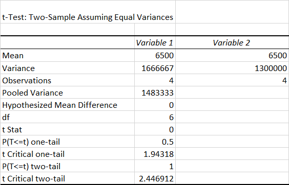
Here’s an explanation of the values in the table from the t-Test: Two-Sample Assuming Equal Variances output:

---

Input Parameters:

1. Mean (6500 for both variables):
   • This is the average value of each sample. Both Variable 1 and Variable 2 have the same mean of 6500.
2. Variance (1666667 and 1300000):
   • This measures the spread of the data in each sample. Variable 1 has a higher variance (1666667) than Variable 2 (1300000), meaning its data points are more spread out from the mean.
3. Observations (4 for each variable):
   • The number of data points in each sample.
4. Pooled Variance (1483333):
   • A weighted average of the variances of the two samples, calculated under the assumption that both populations have equal variances. It combines the information from both samples to estimate the variance.

---

Test Parameters:

5. Hypothesized Mean Difference (0):
   • The assumed difference between the means of the two samples for the null hypothesis. A value of 0 means the test is checking whether the means of the two samples are equal.
6. Degrees of Freedom (df = 6):
   • The degrees of freedom for the test, calculated as: df=n1+n2−2=4+4−2=6df = n_1 + n_2 – 2 = 4 + 4 – 2 = 6
   • This is used to determine the critical t-value.
7. t Stat (0):
   • The calculated t-statistic, which measures the difference between the sample means relative to the variability in the samples. Since both sample means are identical (6500), the t-statistic is 0.

---

Critical Values and p-Values:

8. P(T<=t) one-tail (0.5):
   • The probability of observing a t-statistic as extreme as the calculated value (or more extreme) in one direction under the null hypothesis. A value of 0.5 indicates no significant difference in this case.
9. t Critical one-tail (1.943):
   • The critical t-value for a one-tailed test at the chosen significance level (typically 0.05). If the calculated t-statistic exceeds this value, the null hypothesis is rejected.
10. P(T<=t) two-tail (1):
    • The probability of observing a t-statistic as extreme as the calculated value (or more extreme) in both directions under the null hypothesis. A value of 1 suggests no significant difference.
11. t Critical two-tail (2.447):
    • The critical t-value for a two-tailed test at the chosen significance level (typically 0.05). If the absolute value of the t-statistic exceeds this value, the null hypothesis is rejected.

---

Interpretation:

• The t Stat (0) is smaller than both the critical values (1.943 for one-tail and 2.447 for two-tail).
• The p-values (0.5 for one-tail, 1 for two-tail) are very large, meaning the observed data provides no evidence to reject the null hypothesis.
• Conclusion: There is no significant difference between the means of the two samples.