Table Slicers in Excel

A Table Slicer is an interactive tool in Excel that makes filtering table data visually intuitive. It allows users to filter data in a table or PivotTable by simply clicking on the slicer buttons.

---

Steps to Add and Use Slicers in a Table

1. Create a Table

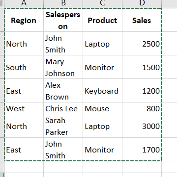
1. Enter data into Excel

1. Convert the data into a table:
   • Highlight the data range.
   • Go to the Insert tab.
   • Click on Table.
   • Check the box for My table has headers, and click OK.

---

2. Insert a Slicer

1. Click anywhere in the table.
2. Go to the Table Design tab (or Table Tools in older versions).
3. Click on Insert Slicer.
4. In the dialog box, select the column(s) you want slicers for (e.g., Region or Salesperson).
5. Click OK.

---

3. Use the Slicer

1. A slicer box will appear with buttons corresponding to the selected column’s values.
2. Click a button (e.g., “North”) to filter the table for rows where the Region is “North.”
3. To clear the filter, click the Clear Filter icon (a funnel with a red X) at the top-right corner of the slicer.

---

Benefits of Slicers

• Ease of Use: Filtering is as simple as clicking buttons.
• Visualization: Shows the filter criteria clearly.
• Multiple Selections: Hold down the Ctrl key (Windows) or Cmd key (Mac) to select multiple values in the slicer.

---

Example

Task: Filter sales data to show rows where the Region is “North” and “East.”

1. Insert a slicer for the Region column.
2. Hold down Ctrl and click North and East in the slicer.

Region	Salesperson	Product	Sales

North

John Smith

Laptop

2500

North

Sarah Parker

Laptop

3000

East

Alex Brown

Keyboard

1200

East

John Smith

Monitor

1700

---

Tips for Slicers

1. Style Slicers:
   • Use the Slicer Tools tab to change the color and style of slicers.
2. Resize and Align:
   • Resize slicers to fit your layout and align them neatly for better presentation.
3. Clear Filters Quickly:
   • Click the Clear Filter button to reset the table.

---